5 Probability distributions in machine learning
This chapter covers
- The role of probability distributions in machine learning
- Working with binomial, multinomial, categorical, Bernoulli, beta, and Dirichlet distributions
- The significance of entropy and cross-entropy in machine learning
Life often requires us to estimate the chances of an event occurring or make a decision in the face of uncertainty. Probability and statistics form the common toolbox to use in such circumstances. In machine learning, we take large feature vectors as inputs. As stated earlier, we can view these feature vectors as points in a high-dimensional space. For instance, gray-level images of size 224 × 224 can be viewed as points in a 50, 176-dimensional space, with each pixel corresponding to a specific dimension. Inputs with common characteristics, such as images of animals, will correspond to a cluster of points in that space. Probability distributions provide an effective tool for analyzing such loosely structured point distributions in arbitrarily high-dimensional spaces. Instead of simply developing a machine that emits a class given an input, we can fit a probability distribution to the clusters of input points (or a transformed version of them) satisfying some property of interest. This often lends more insight into the problem we are trying to solve.
For instance, suppose we are trying to design a recommendation system. We could design one or more classifiers that emit yes/no decisions about whether to recommend product X to person Y. On the other hand, we can fit probability distributions to specific groups of people. Doing so can lead to the discovery of significant overlap between the point clusters representing various groups—for instance, people who drink black coffee and start-up founders. We may not know the explanation or even the direction in which causality (if any) flows in the relationship. But we see the correlation and may design a better recommendation system using it.
Another situation in which probabilistic models are used in machine learning is when the problem involves a very large number of (perhaps infinitely many) classes. For instance, suppose we are creating a machine that not only recognizes cats in an image but also labels each pixel as belonging or not belonging to a cat. Effectively, the machine segments the image pixels into foreground versus background. This is called semantic segmentation. It is hard to cast this problem as a classification problem: we typically design a system that emits a probability of being foreground for each pixel.
Probabilistic models are also used in unsupervised and minimally supervised learning: for instance, in variational autoencoders VAEs), which we discuss in chapter 14.
This chapter introduces the fundamental notion of probability and discusses probability distributions (including multivariates), with specific examples, in a machine learning-centric way. As usual, we emphasize the geometrical view of multivariate statistics. An equally important goal of this chapter is to familiarize you with PyTorch distributions, the PyTorch statistical package, which we use throughout the book. All the distributions discussed are accompanied by code snippets from PyTorch distributions.
NOTE The complete PyTorch code for this chapter is available at http://mng .bz/8NVg in the form of fully functional and executable Jupyter notebooks.
5.1 Probability: The classical frequentist view
Consider a mythical city called Statsville. Suppose we choose a random adult inhabitant of Statsville. What are the chances of this person’s height being greater than 6 ft? Less than 3 ft? Between 5 ft 5 in. and 6 ft? What are the chances of this person’s weight being between 50 and 70 kg (physicists would rather use the term mass here, but we have chosen to stick to the more common word weight)? Greater than 100 kg? What is the probability of the person’s home being exactly 6 km from the city center? What are the chances of the person’s weight being in the 50–70 kg range and their height being in the 5 ft 5 in. to 6 ft range? What are the chances of the person’s weight being greater than 90 kg and their home being within 5 km of the city center?
All these questions can be answered in the frequentist paradigm by adopting the following approach:
Count the size of the population belonging to the desired event satisfying the criterion or criteria of interest): for instance, the number of Statsville adults taller than 6 ft. Divide that by the total size of the population (here, the number of adults in Statsville). This is the probability (chance) of that criterion/criteria being satisfied.
Formally,
Equation 5.1
For instance, suppose there are 100,000 adults in the city. Of them, 25,000 are 6 ft or taller. Then the size of the population satisfying the event of interest (aka the number of favorable outcomes) is 25,000. The total population size (aka the number of possible outcomes) is 100,000. So,
Since the total population is always a superset of the population belonging to any event, the denominator is always greater than or equal to the numerator. Consequently, probabilities are always lesser than or equal to 1.
5.1.1 Random variables
When we talk about probability, a relevant question is, “The probability of what?” The simplest answer is, “The probability of the occurrence of an event.” For example, in the previous subsection, we discussed the probability of the event that the height of an adult Statsville resident is less than 6 ft. A little thought reveals that an event always corresponds to a numerical entity of interest taking a particular value or lying in a particular range of values. This entity is called a random variable. For instance, the height of adult Statsville residents can be a random variable, and we can talk about the probability of it being less than 6 ft, or the weight of adult Statsville residents can be a random variable, and we can talk about the probability of it being less than 60 kg. When predicting the performance of stock markets, the Dow Jones index maybe a random variable: we can talk about the probability of this random variable crossing 19,000. And when discussing the spread of a virus, the total number of infected people may be a random variable, and we can talk about the probability of it being less than 2,000, and so on.
The defining characteristic of a random variable is that every allowed value (or range of values) is associated with a probability (of the random variable taking that value or value range). For instance, we may allow a set of only three weight ranges for adults of Statsville: S1, less than 60 kg; S2, between 60 and 90 kg; and S3, greater than 90 kg. Then we can have a corresponding random variable X representing the quantized weight. It can take one of only three values: X = 1 (corresponding to the weight in S1), X = 2 (corresponding to the weight in S2), or X = 3 (corresponding to the weight in S3). Each value comes with a fixed probability: for example, p(X = 1) = 0.25, p(X = 2) = = 0.5, and p(X = 3) = 0.25, respectively, in the example from section 5.1. Such random variables that take values from a countable set are known as discrete random variables.
Random variables can also be continuous. For a continuous random variable X, we associate a probability with its value being in an infinitesimally small range, p(x ≤ X < x + δx), with δx → 0. This is called probability density and is explained in more detail in section 5.6.
NOTE In this book, we always use uppercase letters to denote random variables. Usually, the same letter in lowercase refers to a specific value of the random variable: for example, p(X = x) denotes the probability of random variable X taking the value x and p(X∈{x, x + δx}) denotes the probability of random variable X taking a value between x and x + δx. Also note that sometimes we use the letter X to denote a data set. This popular but confusing convention is rampant in the literature—generally, the usage is obvious from the context.
5.1.2 Population histograms
Histograms help us to visualize discrete random variables. Let’s continue with our Statsville example. We are only interested in three weight ranges for Statsville adults: S1: less than 60 kg; S2: between 60 and 90 kg; and S3: greater than 90 kg. Suppose the counts of Statsville adults in these weight ranges are as shown in table 5.1.
Table 5.1 Frequency table for the weights of adults in the city of Statsville
|
S1: Less than 60 kg |
S2: Between 60 and 90 kg |
S3: More than 90 kg |
|---|---|---|
|
25,000 |
50,000 |
25,000 |
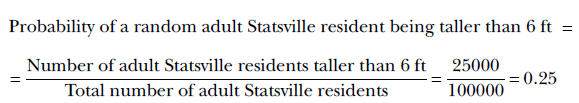
The same information can be visualized by the histogram shown in figure 5.1. The X-axis of the histogram corresponds to possible values of the discrete random variable from section 5.1.1. The Y-axis shows the size of the population in the corresponding weight range. There are 25,000 people in range S1, 50,000 people in range S2, and 25,000 people in range S3. Together, these categories account for the entire adult population of Statsville—every adult belongs to one category or another. This can be verified by adding the Y-axis values for all the categories: 25, 000 + 50, 000 + 25, 000 = 100, 000, the adult population of Statsville.
5.2 Probability distributions
Figure 5.1 and its equivalent, table 5.1, can easily be converted to probabilities, as shown in table 5.2. The table shows the probabilities corresponding to allowed values of the discrete random variable X representing the quantized weight of a randomly chosen adult resident of Statsville. Table 5.2 represents what is formally known as a probability distribution: a mathematical function that takes a random variable as input and outputs the probability of it taking any allowed value. It must be defined over all possible values of the random variable.
Note that the set of ranges {S1, S2, S3} is exhaustive in the sense that all possible values of X belong to one range or other—we cannot have a weight that does not belong to any of them. In set-theoretical terms, the union of these ranges, S1 ∪ S2 ∪ S3, covers a space that contains the entire population (all possible values of X).
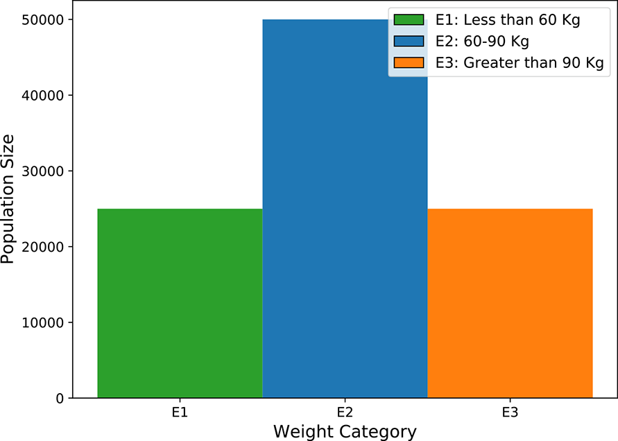
Figure 5.1 Histogram depicting the weights of adults in Statsville, corresponding to table 5.1
Table 5.2 Probability distribution for quantized weights of Statsville adults
|
S1: Less than 60 kg |
S2: Between 60 and 90 kg |
S3: More than 90 kg |
|---|---|---|
| p(X = 1) = 25,000/100,000 = 0.25 | p(X = 2) = 50,000/100,000 = 0.5 | p(X = 3) = 25,000/100,000 = 0.25 |
NOTE The set-theoretic operator ∪ denotes set union.
The ranges are also mutually exclusive in that any given observation of X can belong to only a single range, never more. In set-theoretic terms, the intersection of any pair of ranges is null: S1 ∩ S2 = S1 ∩ S3 = S2 ∩ S3 = ϕ.
NOTE The set-theoretic operator ∩ denotes set intersection.
For a set of exhaustive and mutually exclusive events, the function ielding the probabilities of these events is a probability distribution. For instance, the probability distribution in our tiny example comprises three probabilities: P(X = 1) = 0.25, P(X = 2) = 0.5, and P(X = 3) = 0.25. This is shown in figure 5.2, which is a three-point graph.
Figure 5.2 Probability distribution graph for the weights of adults in Statsville, corresponding to table 5.2. Event E1 ≡ X = 1 ⟹ a weight in the range S1, Event E2 ≡ X = 2 ⟹ a weight in the range S2, and Event E3 ≡ x = 3 ⟹ a weight in the range S3.
5.3 Basic concepts of probability theory
In this section, we briefly touch on impossible and certain events; the sum of probabilities of exhaustive, mutually exclusive events; and independent events.
5.3.1 Probabilities of impossible and certain events
The probability of an impossible event is zero (for example, the probability that the sun will rise in the west). The probability of an event that occurs with certitude is 1 the probability that the sun will rise in the east). Improbable events such as this author beating Roger Federer in competitive tennis) have low but nonzero probabilities, like 0.001. Highly probable events (such as Roger Federer beating this author in competitive tennis) have probabilities close to but not exactly equal to 1, like 0.999.
5.3.2 Exhaustive and mutually exclusive events
Consider the events E1, E2, E3 corresponding to the quantized weight of a Statsville adults from section 5.2 belonging to the range S1, S2, or S3, respectively equivalently, E1 is the event corresponding to X = 1, E2 is the event corresponding to X = 2, and E3 is the event corresponding to X = 3). The events are exhaustive: their union covers the entire population space. This means all quantized weights of Statsville adults belong to one of the ranges S1, S2, S3. The events are also mutually exclusive: their mutual intersections are null, meaning no member of the population can belong to more than one range. For example, if a weight belongs to S1, it cannot belong to S2 or S3. For such events, the following holds true:
The sum of the probabilities of mutually exclusive events yields the probability of one or the other of them occurring.
For instance, for events E1, E2, E3,
p(E1 or E2) = p(E1) + p(E2)
Equation 5.2
the sum rule says that
The sum of the probabilities of an exhaustive, mutually exclusive set of events is always 1.
For example,
p(E1) + p(E2) + p(E3) = p(E1 or E2 or E3) = 1
This is intuitively obvious. We are merely saying that we can say with certainty that either E1 or E2 or E3 will occur.
In general, given a set of exhaustive, mutually exclusive events E1, E2, ⋯, En,
Equation 5.3
5.3.3 Independent events
Consider the two events E1 ≡ “weight of an adult inhabitant of Statsville is less than 60 kg” and G1 ≡ “home of an adult inhabitant of Statsville is within 5 km of the city center”. These events do not influence each other at all. The knowledge that a member of the population weighs less than 60 kg does not reveal anything about the distance of their home from the city center and vice versa. We say E1 and G1 are independent events. Formally,
A set of events are independent if the occurrence of one does not affect the probability of the occurrence of another.
5.4 Joint probabilities and their distributions
Given an adult Statsville resident, let E1 be, as before, the event that their weight is less than 60 kg. The corresponding probability is p(E1). Also, let G1 be the event that the distance of their home from the city center is less than 5 km. The corresponding probability is p(G1). Now consider the probability that a resident weights less than 60 kg and their home is less than 5 km from the city center. This probability, denoted p(E1, G1), is called a joint probability. Formally,
The joint probability of a set of events is the probability of all those events occurring together.
The product rule says that the joint probability of independent events can be obtained by multiplying their individual probabilities. Thus, for the current example, p(E1, G1) = p(E1)p(G1).
Let’s continue our discussion of joint probabilities with a slightly more elaborate example. We have consolidated the weight categories, corresponding populations, and probability distributions in table 5.3 for quick reference. Similarly, we quantize the distance of residents’ homes from the city center into three ranges: D1 ≡ less than 5 km, D2 ≡ between 5 and 15 km, and D3 ≡ greater than 15 km. Table 5.4 shows the corresponding population and probability distributions. The joint probability distribution of the events {E1, E2, E3} and {G1, G2, G3} is shown in table 5.5.
Table 5.3 Population probability distribution table for the weights of adult residents of Statsville. E1, E2, E3 are exhaustive, mutually exclusive events, p(E1) + p(E2) + p(E3) = 1.
|
Less than 60 kg (range S1) |
Between 60 and 90 kg (range S2) |
More than 90 kg (range S3) |
|---|---|---|
|
Event E1 ≡ weight ∈ S1 |
Event E2 ≡ weight ∈ S2 |
Event E3 ≡ weight ∈ S3 |
|
Population size = 25,000 |
Population size = 50,000 |
Population size = 25,000 |
|
p(S1) = 25,000/100,000 = 0.25 |
p(S2) = 50,000/100,000 = 0.5 |
p(S3) = 25,000/100,000 = 0.25 |
Table 5.4 Population probability distribution table for the distance of adult Statsville residents’ homes from the city center. G1, G2, G3 are exhaustive, mutually exclusive events, p(G1) + p(G2) + p(G3) = 1.
|
Less than 5 km (range D1) |
Between 5 and 15 km (range D2) |
Greater than 15 km (range D3) |
|---|---|---|
|
Event G1 ≡ distance ∈ D1 |
Event G2 ≡ distance ∈ D2 |
Event G3 ≡ distance ∈ D3 |
|
Population size = 20,000 |
Population size = 60,000 |
Population size = 20,000 |
|
p(G1) = 20,000/100,000 = 0.20 |
p(G1) = 60,000/100,000 = 0.6 |
p(G1) = 20,000/100,000 = 0.20 |
Table 5.5 Joint probability distribution of independent events. The sum of all elements in the table is 1.
|
|
Less than 60 kg (E1) |
Between 60 and 90 kg (E2) |
More than 90 kg (E3) |
|---|---|---|---|
|
Less than 5 km (G1) |
p(E1, G1) = 0.25 × 0.2 = 0.05 |
p(E2, G1) = 0.5 × 0.2 = 0.1 |
p(E3, G1) = 0.25 × 0.2 = 0.05 |
|
Between 5 and 15 km (G2) |
p(E1, G2) = 0.25 × 0.6 = 0.15 |
p(E2, G2) = 0.5 × 0.6 = 0.3 |
p(E3, G2) = 0.25 × 0.6 = 0.15 |
|
More than 15 km (G3) |
p(E1, G3) = 0.25 × 0.2 = 0.05 |
p(E2, G3) = 0.5 × 0.2 = 0.1 |
p(E3, G3) = 0.25 × 0.2 = 0.05 |
We can make the following statements about table 5.5:
-
The sum total of all elements in table 5.5 is 1. In other words, p(Ei, Gj) is a proper probability distribution indicating the probabilities of event Ei and event Gj occurring together: here, (i, j) ∈ {1,2,3} × {1,2,3}.
-
p(Ei, Gj) = p(Ei)p(Gj) ∀(i, j) ∈ {1,2,3} × {1,2,3}. This is because the events are independent.
NOTE The symbol × denotes the Cartesian product. The Cartesian product of two sets {1,2,3} × {1,2,3} is the set {(1,1),(1,2),(1,3),(2,1),(2,2),(2,3),(3,1),(3,2),(3,3)}. And the symbol ∀ indicates “for all.” Read ∀(i, j) ∈ {1,2,3} × {1,2,3} as follows: for all pairs (i, j) in the Cartesian product, {1,2,3} × {1,2,3}.
In general, given a set of independent events E1, E2, ⋯, En, the joint probability p(E1, E2,⋯, En) of all the events occurring together is the product of their individual probabilities of occurring:
Equation 5.4
NOTE The symbol ∏ stands for “product.”
5.4.1 Marginal probabilities
Suppose we do not have the individual probabilities p(Ei) and p(Gj). All we have is the joint probability distribution: that is, table 5.5. Can we find the individual probabilities from them? If so, how?
To answer this question, consider a particular row or column in table 5.5—say, the top row. In this row, the E values iterate over all possibilities (the entire space of Es), but G is fixed at G1. If G1 is to occur, there are only three possibilities: it occurs with E1, E2, or E3. The corresponding joint probabilities are p(E1, G1), p(E2, G1), and p(E3, G1). If we add them, we get the probability of G1 occurring with E1 or E2, or E3: that is, event (E1, G1) or (E2, G1) or (E3, G1). Thus we have considered all situations under which G1 can occur. The sum represents the probability of event G1 occurring. Thus, p(G1) can be obtained by adding all the probabilities in the row corresponding to G1 and writing it in the margin (this is why it is called the marginal probability). Similarly, by adding all the probabilities in the middle column, we obtain the probability p(E2), and so forth. Table 5.6 shows table 5.5 updated with marginal probabilities.
Table 5.6 Joint probability distribution with marginal probabilities shown
|
Less than 60 kg (E1) |
Between 60 and 90 kg (E2) |
More than 90 kg (E3) |
Marginals for G’s |
|
|---|---|---|---|---|
|
Less than 5 km (G1) |
p(E1, G1) = 0.25 × 0.2 = 0.05 |
p(E2, G1) = 0.5 × 0.2 = 0.1 |
p(E3, G1) = 0.25 × 0.2 = 0.05 |
p(G1) = 0.05 + 0.1 + 0.05 = 0.2 |
|
Between 5 and 15 km (G2) |
p(E1, G2) = 0.25 × 0.6 = 0.15 |
p(E2, G2) = 0.5 × 0.6 = 0.3 |
p(E3, G2) = 0.25 × 0.6 = 0.15 |
p(G2) 0.15 + 0.3 + 0.15 = 0.6 |
|
More than 15 km (G3) |
p(E1, G3) = 0.25 × 0.2 = 0.05 |
p(E2, G3) = 0.5 × 0.2 = 0.1 |
p(E3, G3) = 0.25 × 0.2 = 0.05 |
p(G3) = 0.05 + 0.1 + 0.05 = 0.2 |
|
Marginals for Es |
p(E1) = 0.05 + 0.15 + 0.05 0.05 = 0.25 |
p(E2) = 0.1 + 0.3 + 0.1 = 0.5 |
p(E3) = 0.05 + 0.15 + = 0.25 |
In general, given a set of exhaustive, mutually exclusive events E1, E2, ⋯, En, another event G, and joint probabilities p(E1, G), p(E2, G), ⋯, p(En, G),
Equation 5.5
By summing over all possible values of Eis, we factor out the Es. This is because the Es are mutually exclusive and exhaustive; summing over them results in a certain event that is factored out (remember, the probability of a certain event is 1).
5.4.2 Dependent events and their joint probability distribution
So far, the events we have considered jointly are “weights” and “distance of a resident’s home from the city center.” These are independent of each other—their joint is the product of their individual probabilities. Now, let’s discuss a different situation where the variables are connected and knowing the value of one does help us predict the other. For instance, the weights and heights of adult residents of Statsville are not independent: typically, taller people weigh more, and vice versa.
As usual, we use a toy example to understand the idea. We quantize heights into three ranges, H1 ≡ less than 5 ft 5 in., H2 ≡ between 5 ft 5 in. and 6 ft, and H3 ≡ greater than 6 ft. Let z be the random variable corresponding to height. We have three possible events with respect to height: F1 ≡ z ∈ H1, F2 ≡ z ∈ H2, and F3 ≡ z ∈ H3. The joint probability distribution of height and weight is shown in table 5.7.
Table 5.7 Joint probability distribution of dependent events
|
Less than 60 kg (E1) |
Between 60 and 90 kg (E2) |
More than 90 kg (E3) |
|
|---|---|---|---|
|
Less than 5 ft 5 in. (F1) |
p(E1, F1) = 0.25 |
p(E2, F1) = 0 |
p(E3, F1) = 0 |
|
Between 5 ft 5 in. and 6 ft (F2) |
p(E1, F2) = 0. |
p(E2, F2) = 0.5 |
p(E3, F2) = 0 |
|
More than 6 ft (F3). |
p(E1, F3) = 0 |
p(E2, F3) = 0 |
p(E3, F3) = 0.25 |
Note the following about table 5.7:
-
The sum total of all elements in table 5.7 is 1. In other words, p(Ei, Fj) is a proper probability distribution indicating the probabilities of event Ei and event Fj occurring together. Here (i, j) ∈ {1,2,3} × {1,2,3}.
-
p(Ei, Fj) = 0 if i ≠ j ∀(i, j) ∈ {1,2,3} × {1,2,3}. This essentially means the events are perfectly correlated: the occurrence of E1 implies the occurrence of F1 and vice versa, the occurrence of E2 implies the occurrence of F2 and vice versa, and the occurrence of E3 implies the occurrence of F3 and vice versa. In other words, every adult resident of Statsville who weighs less than 60 kg is also shorter than 5 ft 5 in., and so on. (In life, such perfect correlations rarely exist; but Statsville is a mythical town.)
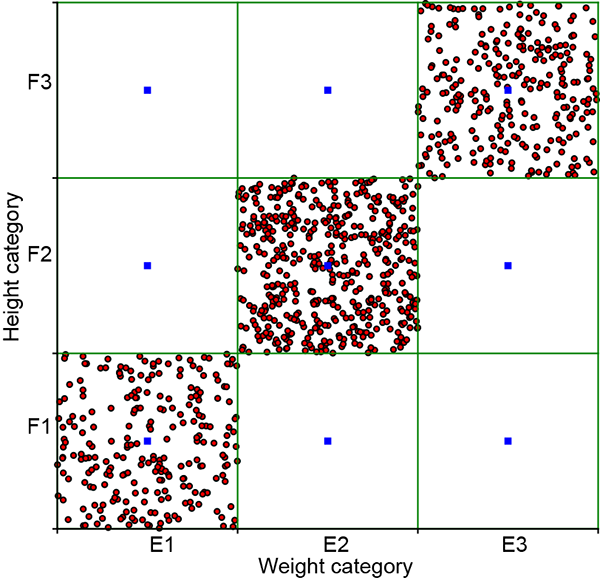
5.5 Geometrical view: Sample point distributions for dependent and independent variables
Let’s look at a graphical view of the point distributions corresponding to tables 5.5 and 5.7. There is a fundamental difference in how the point distributions look for independent and dependent variables; it is connected to principal component analysis (PCA) and dimensionality reduction, which we discussed in section 4.4.
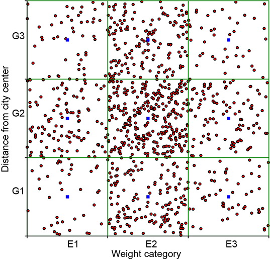
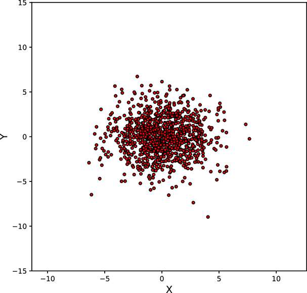
We use a rectangular bucket-based technique to visualize joint 2D discrete events. For instance, we have three weight-related events, E1, E2, E3, and three distance-related events, G1, G2, G3. Hence the joint distribution has 3 × 3 = 9 possible events (Ei, Gj), ∀(i, j) ∈ {1,2,3} × {1,2,3}, as shown in table 5.5. Each of these nine events is represented by a small rectangle (bucket for the joint event); altogether, we have a 3 × 3 grid of rectangular buckets. To visualize the sample point distribution, we have drawn 1,000 samples from the joint distribution. A joint event sample is placed at a random location within its bucket (that is, all points within the bucket have an equal probability of being selected). Notice that the concentration of points is greater inside high-probability buckets and vice versa.
(a)
(b)
Figure 5.3 Graphical visualization of joint probability distributions. Rectangles represent buckets of different discrete events. (a) From table 5.5 independent events). The probabilities of all nine events are non-negligible, and all nine rectangles have a relatively high concentration of sample points. Not suitable for PCA. (b) From table 5.7 (non-independent events). Events (E1, F1), (E2, F2), and (E3, F3) have very high probabilities, and other events have negligible probabilities. Sample points are concentrated along the rectangles on the diagonal. Suitable for PCA.
Graphical views of the point distribution for the independent table 5.5) and non-independent table 5.7) joint variable pairs are shown in figures 5.3a and 5.3b, respectively. We see that the sample point distribution for the independent events is spread somewhat symmetrically over the domain, while that for the dependent events is spread narrowly around a particular line (in this case, the diagonal). This holds true in general and for higher dimensions, too. You should have this mental picture with respect to independent versus non-independent point distributions. If we sample independent events (uncorrelated), all possible combinations of events {E1, G1}, {E1, G2}, {E1, G3}, ⋯, {E3, G3} have a non-negligible probability of occurrence (see table 5.5), which is equivalent to saying that none of the events have a very high probability of occurring remember that probabilities sum to 1, so if some events have very low probabilities [close to zero], other events must have high probabilities [near one] to compensate). This precludes the concentration of points in a small region of the space. All buckets will have many points. In other words, the joint probability samples of independent events are diffused throughout the population space (see figure 5.3a, for instance).
On the other hand, if the events are correlated, the joint probability samples are concentrated in certain high-probability regions of the joint space. For instance, in table 5.7, events (E1, F1), (E2, F2), (E3, F3) are far more likely than the other combinations. Hence, the sample points are concentrated along the corresponding diagonal (see figure 5.3b).
If this does not remind you of PCA (section 4.4), you should re-read that section. Dependent events such as that shown in figure 5.3a are good candidates for dimensionality reduction: the two dimensions essentially carry the same information, and if we know one, we can derive the other. We can drop one of the highly correlated dimensions without losing significant information.
5.6 Continuous random variables and probability density
So far, we have quantized our random variables and made them discrete. For instance, weight has been quantized into three buckets—less than 60 kg, between 60 and 90 kg, and greater than 90 kg—and probabilities have been assigned to each bucket. What if we want to know probabilities at a more granular level like 0 to 10 kg, 10 to 20 kg, 20 to 30 kg, and so on? Well, we have to create more buckets. Each bucket covers a narrower range of values (a smaller portion of the population space), but there are more of them. In all cases, following the frequentist approach, we count the number of adult Statsvilleans in each bucket, divide that by the total population size, and call that the probability of belonging to that bucket.
What if we want even further granularity? We create even more buckets, each covering an even smaller portion of the population space. In the limit, we have an infinite number of buckets, each covering an infinitesimally small portion of the population space. Together they still cover the population space—a very large number of very small pieces can cover arbitrary regions. At this limit, the probability distribution function is called a probability density function. Formally,
The probability density function p(x) for a continuous random variable X is defined as the probability that X lies between x and x + δx with δx → 0
p(x) = limδx→0 probability(x ≤ X < x + δx)
NOTE It is slightly unfortunate that the typical symbol for a random variable, X, collides with that for a dataset (collection of data vectors), also X. But the context is usually enough to tell them apart.
There is a bit of theoretical nuance here. We are saying that p(x) is the probability of the random variable X lying between x and x + δx. This is not exactly the same as saying that p(x) is the probability that X is equal to x. But because δx is infinitesimally small, they amount to the same thing.
Consider the set of events E = limδx→0 {x ≤ X < x + δx} for all possible values of x. All possible values of x range from negative infinity to infinity: x ∈ [−∞,∞]. There are infinite such events, each of which is infinitesimally narrow, but together they cover the entire domain x ∈ [−∞,∞]. In other words, they are exhaustive. They are also mutually exclusive because x cannot belong to more than one of them at the same time. They are continuous counterparts of the discrete events E1, E2, E3 that we have seen before.
The fact that the set of events E = limδx → 0{x ≤ X < x + δx} in continuous space is exhaustive and mutually exclusive means we can apply equation 5.3 but the sum will be replaced by an integral as the variable is continuous.
The sum rule in a continuous domain is expressed as
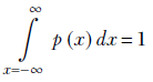
Equation 5.6
Equation 5.6 is the continuous analog of equation 5.3. It physically means we can say with certainty that x lies somewhere in the interval −∞ to ∞.
The random variable can also be multidimensional (that is, a vector). Then the probability density function is denoted as p(![]() ).
).
The sum rule for a continuous multidimensional probability density function is
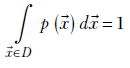
Equation 5.7
where D is the domain of ![]() —that is, the space containing all possible values of the vector
—that is, the space containing all possible values of the vector ![]() .
.
For instance, the 2D vector ![]() has the XY plane as its domain. Note that the integral in equation 5.7 is a multidimensional integral (for example, for 2D
has the XY plane as its domain. Note that the integral in equation 5.7 is a multidimensional integral (for example, for 2D ![]() , it is ∬
, it is ∬![]() ∈D p(
∈D p(![]() ) d
) d![]() = 1).
= 1).
NOTE For simplicity of notation, we usually use a single integral sign to denote multidimensional integrals. The vector sign in the domain (for example, ![]() ∈ D), as well the vector sign in d
∈ D), as well the vector sign in d![]() , indicates multiple dimensions.
, indicates multiple dimensions.
You may remember from elementary integral calculus that equation 5.6 corresponds to the area under the curve for p(x) (or p(![]() )). In higher dimensions, equation 5.7 corresponds to the volume under the hypersurface for p(
)). In higher dimensions, equation 5.7 corresponds to the volume under the hypersurface for p(![]() ). Thus, the total area under a univariate probability density curve is always 1. And in higher dimensions, the volume under the hypersurface for a multivariate probability density function is always 1.
). Thus, the total area under a univariate probability density curve is always 1. And in higher dimensions, the volume under the hypersurface for a multivariate probability density function is always 1.
5.7 Properties of distributions: Expected value, variance, and covariance
Toward the beginning of this chapter, we stated that generative machine learning models are often developed by fitting a distribution from a known family to the available training data. Thus, we postulate a parameterized distribution from a known family and estimate the exact parameters that best fit the training data. Most distribution families are parameterized in terms of intuitive properties like the mean, variance, and so on. Understanding these concepts and their geometric significance is essential for understanding the models based on them.
In this section, we explain a few properties/parameters common to all distributions. Later, when we discuss individual distributions, we connect them to the parameters of those distributions. We also show how to programmatically obtain the values of these for each individual distribution via the PyTorch distributions package.
5.7.1 Expected value (aka mean)
If we sample a random variable with a given distribution many times and take the average of the sampled values, what value do we expect to end up with? The average will be closer to the values with higher probabilities (as these appear more often during sampling). If we sample enough times, for a given probability distribution, this average always settles down to a fixed value for that distribution: the expected value of the distribution.
Formally,
given a discrete distribution D where a discrete random variable X can take any value from the sets {x1, x2,⋯, xn} with respective probabilities {p(x1), p(x2)⋯, p(xn)}, the expected value is given by the formula
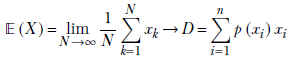
Equation 5.8
where xk → D denotes the kth sample drawn from the distribution D. Overall, equation 5.8 says that the average or expected value of a very large number of samples drawn from the distribution approaches the probability-weighted sum of all possible sample values. When we sample, the higher-probability values appear more frequently than the lower-probability values, so the average over a large number of samples is pulled closer to the higher-probability values.
For multivariate random variables:
Given a discrete distribution where a discrete multidimensional random variable X can take any value from the sets {![]() 1,
1, ![]() 2,⋯,
2,⋯, ![]() n} with respective probabilities {p(
n} with respective probabilities {p(![]() 1), p(
1), p(![]() 2),⋯, p(
2),⋯, p(![]() n)}, the expected value is given by the formula
n)}, the expected value is given by the formula

Equation 5.9
For continuous random variables (note how the sum is replaced by an integral):
The expected value of a continuous random variable X that takes values from −∞ to ∞ (that is, x ∈ { − ∞, ∞}) is
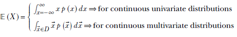
Equation 5.10
Expected value and center of mass in physics
In physics, we have the concept of the center of mass or centroid. If we have a set of points, each with a mass, the entire point set can be replaced by a single point. This point is called the centroid. The position of the centroid is the weighted average of the positions of the individual points, weighted by their individual masses. If we mentally think of the probabilities of individual points as masses, the notion of expected value in statistics corresponds to the notion of centroid in physics.
Expected value of an arbitrary function of a random variable
So far, we have seen the expected value of the random variable itself. The notion can be extended to functions of the random variable.
The expected value of a function of a random variable is the probability-weighted sum of the values of that function at all possible values of the random variable. Formally,
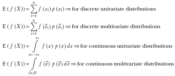
Equation 5.11
Expected value and dot product
In equation 2.6, we looked at the dot product between two vectors. Further, in section 2.5.6.2, we saw that the dot product between two vectors measures the agreement between the two vectors. If both point in the same direction, the dot product is larger. In this section, we show that the expected value of a function of a random variable can be viewed as a dot product between a vector representing the probability and another vector representing the function itself.
First let’s consider the discrete case. Our random variable can take values xi, i ∈ {1, n}. Now, imagine a vector  and a vector
  . From equation 5.11, we see that the expected value of the function 𝔼(f(X)) of random variable X is the same as
 ![]() T
T![]() =
= ![]() ⋅
⋅ ![]() . This is high when
. This is high when ![]() and
and ![]() are aligned; thus, the expected value of the function of the random variable is high when the high function values coincide with high probabilities of the random variable and vice versa. In the continuous case, these vectors have an infinite number of components and the summation is replaced by an integral, but the idea stays the same.
are aligned; thus, the expected value of the function of the random variable is high when the high function values coincide with high probabilities of the random variable and vice versa. In the continuous case, these vectors have an infinite number of components and the summation is replaced by an integral, but the idea stays the same.
Expected value of linear combinations of random variables
The expected value is a linear operator. This means the expected value of a linear combination of random variables is a linear combination (with the same weights) of the expected values of the random variables. Formally,
𝔼(α1X1 + α2X2 ⋯ αnXn) = α1𝔼(X1) + α2𝔼(X2) + ⋯ αn𝔼(Xn)
Equation 5.12
5.7.2 Variance, covariance, and standard deviation
When we draw a very large number of samples from a given point distribution, we often like to know the spread of the point set. The spread is not merely a matter of measuring the largest distance between two points in the distribution. Rather, we want to know how densely packed the points are. If most of the points fit within a very small ball, then even if one or two points are far from the ball, we call that a small spread or high packing density.
Why is this important in machine learning? Let’s start with a few informal examples. If we discover that the points are tightly packed in a small region around a single point, we may want to replace the entire distribution with that point without causing much error. Or if the points are packed tightly around a single straight line, we can replace the entire distribution with that line. Doing so gives us a simpler lower-dimensional) representation and often leads to a view of the data that is more amenable to understanding the big picture. This is because small variations about a particular point or direction are usually caused by noise, while large variations are caused by meaningful things. By eliminating small variations and focusing on the large ones, we capture the main information content. (This could be why older people tend to be better at forming big-picture views: perhaps there are too few neurons in their heads to retain the huge amount of memory data they have accumulated over the years. Their brain performs dimensionality reduction.) This is the basic idea behind PCA and dimensionality reduction, which we saw in section 4.4.
Variance—or its square root, standard deviation—measures how densely packed around the expected value the points in the distribution are: that is, the spread of the point distribution. Formally, the variance of a probability distribution is defined as follows:
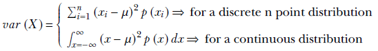
Equation 5.13
By comparing equation 5.13 to equations 5.10 and 5.11, we see that the variance is the expected value of the distance (x − μ)2 of sample points x from the mean μ. So if the more probable (more frequently occurring) sample points lie within a short distance of the mean, the variance is small, and vice versa. That is to say, the variance measures how tightly packed the points are around the mean.
Covariance: Variance in higher dimensions
Extending the notion of the expected value from the univariate case to the multivariate case was straightforward. In the univariate case, we take a probability-weighted average of a scalar quantity, x. The resulting expected value is a scalar, μ = ∫x = −∞∞ x p(x)dx. In the multivariate case, we take the probability-weighted average of a vector quantity, ![]() . The resulting expected value is a vector,
. The resulting expected value is a vector, ![]() = ∫
= ∫![]() ∈D
∈D ![]() p(
p(![]() )d
)d![]() .
.
Extending the notion of variance to the multivariate case is not as straightforward. This is because we can traverse the multidimensional random vector’s domain (the space over which the vector is defined) in an infinite number of possible directions—think how many possible directions we can walk on a 2D plane—and the spread or packing density can be different for each direction. For instance, in figure 5.3b, the spread along the main diagonal is much larger than the spread in a perpendicular direction.
The covariance of a multidimensional point distribution is a matrix that allows us to easily measure the spread or packing density in any desired direction. It also allows us to easily figure out the direction in which the maximum spread occurs and what that spread is.
Consider a multivariate random variable X that takes vector values ![]() . Let l̂ be an arbitrary direction (as always, we use overhead hats to denote unit-length vectors signifying directions) in which we want to measure the packing density of X. We discussed in sections 2.5.2 and 2.5.6 that the dot product of
. Let l̂ be an arbitrary direction (as always, we use overhead hats to denote unit-length vectors signifying directions) in which we want to measure the packing density of X. We discussed in sections 2.5.2 and 2.5.6 that the dot product of ![]() in the direction l̂ (that is,
in the direction l̂ (that is, ![]() Tl̂) is the projection or component (effective value) of x along l̂. Thus the spread or packing density of the random vector
Tl̂) is the projection or component (effective value) of x along l̂. Thus the spread or packing density of the random vector ![]() in direction l̂ is the same as the spread of the dot product (aka component or projection) l̂T
in direction l̂ is the same as the spread of the dot product (aka component or projection) l̂T![]() . This projection l̂T
. This projection l̂T![]() is a scalar quantity: we can use the univariate formula to measure its variance.
is a scalar quantity: we can use the univariate formula to measure its variance.
NOTE In this context, we can use ![]() Tl̂ and l̂T
Tl̂ and l̂T![]() interchangeably. The dot product is symmetric.
interchangeably. The dot product is symmetric.
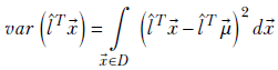
The expected value of the projection is
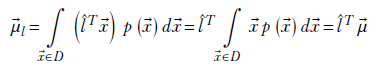
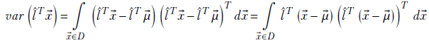
The variance is given by
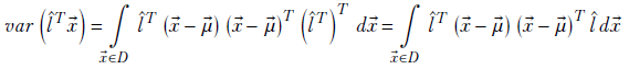
Now, since the transpose of a scalar is the same scalar, we can write the square term within the integral as the product of the scalar l̂T(![]() -
- ![]() ) and its transpose:
) and its transpose:
Using equation 2.10,
Since
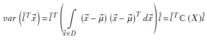
where
Equation 5.14
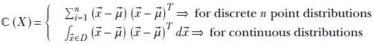
For simplicity, we drop the X in parentheses and simply write ℂ(X) as ℂ. An equivalent way of looking at the covariance matrix of a d-dimensional random variable X taking vector values ![]() is as follows:
is as follows:
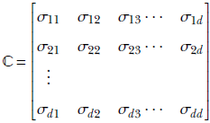
Equation 5.15
where
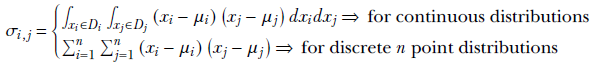
is the co-variance of the ith and jth dimensions of the random vector ![]() .
.
ℂ(X) or ℂ is the covariance matrix of the random variable X. A little thought reveals that equations 5.14 and 5.15 are equivalent.
The following things are noteworthy:
-
From equation 5.14, ℂ is the sum of the products of d × 1 vectors (
 −
− ) and their transpose (−)T, 1 × d vectors. Hence, ℂ is a d × d matrix.
 -
This matrix is independent of the direction, l̂, in which we are measuring the variance or spread. We can precompute ℂ; then, when we need to measure the variance in any direction l̂, we can evaluate the quadratic form l̂T ℂl̂ to obtain the variance in that direction. Thus ℂ is a generic property of the distribution, much like
. ℂ is called the covariance of the distribution. -
Covariance is the multivariate peer of the univariate entity variance.
That covariance is the multivariate analog of variance is evident by comparing the expressions in equations 5.13 and 5.14.
Variance and expected value
As outlined previously, the variance is the expected value of the distance (x − μ)2 of sample points x from the mean μ. This can be easily seen by comparing equations 5.13, 5.10, and 5.11 and leads to the following formula (where we use the principle of the expected value of linear combinations):
var(X) = 𝔼((X − μ)2) = 𝔼(X2) − 𝔼(2μX) + 𝔼(μ2)
Since μ is a constant, we can take it out of the expected value (a special case of the principal of the expected value of linear combinations). Thus we get
var(X) = 𝔼(X2) − 2μ𝔼(X) + μ2𝔼(1)
But μ = 𝔼(X). Also, the expected value of a constant is that constant. So, 𝔼(1) = 1.
Hence,
var(X) = 𝔼(X2) − 2μ2 + μ2𝔼(1) = 𝔼(X2) − μ2
or
var(X) = 𝔼(X2) − 𝔼(X)2
Equation 5.16
5.8 Sampling from a distribution
Drawing a sample from the probability distribution of a random variable yields an arbitrary value from the set of possible values. If we draw many samples, the higher-probability values show up more often than lower-probability values. The sampled points form a cloud in the domain of possible values, and the region where the probabilities are higher is more densely populated than lower-probability regions. In other words, in a sample point cloud, higher-probability values are overrepresented. Thus a collection of sample points is often referred to as a sample point cloud. The hope, of course, is that the sample point cloud is a good representation of the entire population so that analyzing the points in the cloud will yield insights about the entire population. In univariate cases, the sample value is a scalar and represented by a point on the number line. In multivariate cases, the sample value is a vector and represented as a point in a higher-dimensional space.
It is often useful to compute aggregate statistics (such as the mean and variance) to describe the population. If we know a distribution, we can use closed-form expressions to obtain these properties. Many standard distributions and closed-form equations for obtaining their means and variance are discussed in section 5.9. But often, we don’t know the underlying distribution. Under those circumstances, the sample mean and sample variance can be used. Given a set of n samples X = ![]() 1,
1, ![]() 2⋯
2⋯![]() n from any distribution, the sample mean and variance are computed as
n from any distribution, the sample mean and variance are computed as
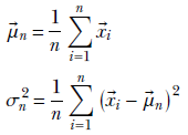
In some situations, like Gaussian distributions (which we discuss shortly), it can be theoretically proved that the sample mean and variance are optimal (the best possible guesses of the true mean and variance, given the sampled data). Also, the sample mean approaches the true mean as the number of samples increases, and with enough samples, we get a pretty good approximation of the true mean. In the next subsection, we learn more about how much is “enough.”
Law of large numbers: How many samples are enough?
Informally speaking, the law of large numbers says that if we draw a large number of sample values from a probability distribution, their average should be close to the expected value of the distribution. In the limit, the average over an infinite number of samples will match the mean.
In practice, we cannot draw an infinite number of samples, so there is no guarantee that the sample mean will coincide with the expected value (true mean) in real-life sampling. But if the number of samples is large, they will not be too different. This is not a matter of mere theory. Casinos design games where the probability of the house winning a bet against the guest is slightly higher than the probability of the guest winning. The expected value of the outcome is that the casino wins rather than the guest. Over the very large number of bets placed in a casino, this is exactly what happens—and that is why casinos make money on the whole, even though they may lose individual bets.
How many samples is “a large number of samples?” Well, it is not defined precisely. But one thing is known: if the variance is larger, more samples need to be drawn to make the law of large numbers apply.
Let’s illustrate this with an example. Consider a betting game. Suppose that the famous soccer club FC Barcelona, for unknown reasons, has agreed to play a very large number of matches against the Machine Learning Experts’ Soccer Club of Silicon Valley. We can place a bet of $100 on a team. If that team wins, we get back $200: that is, we make $100. If that team loses, we lose the bet: that is, we make –$100. The betting game is happening in a country where nobody knows anything about the reputations of these clubs. A bettor bets on FC Barcelona in the first game and wins $100. Based on this one observation, can the bettor say that by betting on Barcelona, they expect to win $100 every time? Obviously not.
But suppose the bettor places 100 bets and wins $100 99 times and loses $100 once. Now the bettor can expect with some confidence that they will win $100 (or close to it) by betting on Barcelona. Based on these observations, the sample mean winnings from a bet on FC Barcelona are 0.99 × (100) + 0.01 × (−100) = 98. The sample standard deviation is √(.99 × (98 - 100)2 + 0.01 × (98 - (-100))2) = 19.8997. Relative to the sample mean, the sample standard deviation is 19.8997/98 = 0.203.
Next, consider the same game, except now FC Barcelona is playing the Real Madrid football club. Since the two teams are evenly matched (the theoretical win probability of Barcelona is 0.5), the results are no longer one-sided. Suppose that after 100 games, FC Barcelona has won 60 times and Real Madrid has won 40 times. The sample mean winnings on a Barcelona bet are 0.6 × (100) + 0.4 × (−100) = 20. The sample standard deviation is √(.6 × (20 - 100)2 + 0.4 × (20 - (-100))2) = 97.9795. Relative to the sample mean, the sample standard deviation is 97.9795/20 = 4.89897. This is a much larger number than the previous 0.203. In this case, even after 100 trials, a bettor cannot be very confident in predicting that the expected win is the sample mean, $20.
The overall intuition is as follows:
If we take a sufficiently large number of samples, their average is close to the expected value. The exact definition of what constitutes a “sufficiently large” number of samples is not known. However, the larger the variance (relative to the mean), the more samples are needed.
5.9 Some famous probability distributions
In this section, we introduce some probability distributions and density functions often used in deep learning. We will use PyTorch code snippets to demonstrate how to set up, sample, and compute properties like expected values, variance/covariance, and so on for each distribution. Note the following:
-
In the code snippets, for every distribution, we evaluate the probability using
-
A PyTorch
distributionsfunction call -
A raw evaluation from the formula (to understand the math)
Both should yield the same result. In practice, you should use the PyTorch
distributionsfunction call instead of the raw formula. -
-
In the code snippets, for every distribution,
-
We evaluate the theoretical mean and variance using a PyTorch
distributionsfunction call. -
We evaluate the sample mean and variance.
When the sample set is large enough, the sample mean and theoretical mean should be close. Ditto for variance.
-
NOTE Fully functional code for these distributions, executable via Jupyter Notebook, can be found at http://mng.bz/8NVg.
Another point to remember: In machine learning, we often work with the logarithm of the probability. Since the popular distributions are exponential, this leads to simpler computations. With that, let’s dive into the probability distributions.
5.9.1 Uniform random distributions
Consider a continuous random variable x that can take any value from a fixed compact range, say [a, b], with equal probability, while the probability of x taking a value outside the range is zero. The corresponding p(x) is a uniform probability distribution. Formally stated,
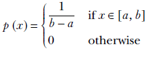
Equation 5.17
Equation 5.17 means p(x) is constant, 1/b-a, for x between a and b and zero for other values of x. Note how the value of the constant is cleverly chosen to make the total area under the curve 1. This equation is depicted graphically in figure 5.4, and listing 5.1 shows the PyTorch code for the log probability of a univariate uniform random distribution.
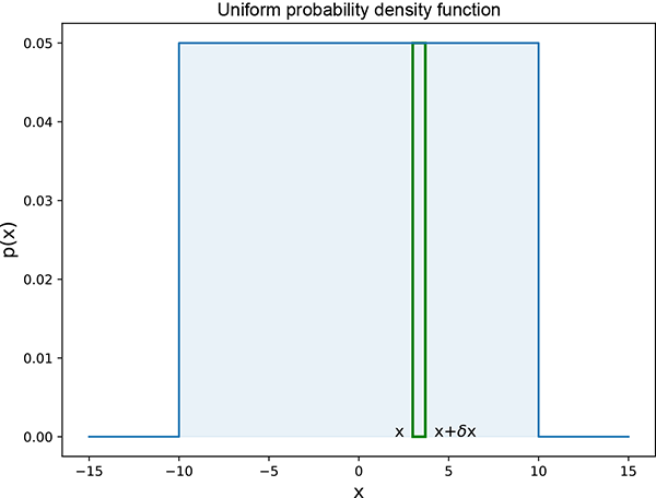
Figure 5.4 Univariate (single-variable) uniform random probability density function. Probability p(x) is constant, 0.05, in the interval [−10,10] and zero everywhere outside the interval. Thus it depicts equation 5.17 with b = 10, a = −10. The area under the curve is the area of the shaded rectangle of width 20 and height 0.05, 20 × 0.05 = 1. The thin rectangle depicts an infinitesimally small interval corresponding to event E = {x ≤ X < x + δx}. If we draw a random sample x from this distribution, the probability that the value of the sample is between, say, 4 and 4 + δx, with δx → 0, is p(4) = 0.05. The probability that the value of the sample is between, say, 15 and 15 + δx, with δx → 0, is p(15) = 0.
Listing 5.1 Log probability of a univariate uniform random distribution
from torch.distributions import Uniform                      ①

a = torch.tensor([1.0], dtype=torch.float)                   ②
b = torch.tensor([5.0], dtype=torch.float)

ufm_dist = Uniform(a, b)                                     ③

X = torch.tensor([2.0], dtype=torch.float)                   ④

def raw_eval(X, a, b):
    return torch.log(1 / (b - a))

log_prob = ufm_dist.log_prob(X)                              ⑤

raw_eval_log_prob = raw_eval(X, a, b)                        ⑥

assert torch.isclose(log_prob, raw_eval_log_prob, atol=1e-4) ⑦
① Imports a PyTorch uniform distribution
② Sets the distribution parameters
③ Instantiates a uniform distribution object
④ Instantiates a single-point test dataset
⑤ Evaluates the probability using PyTorch
⑥ Evaluates the probability using the formula
⑦ Asserts that the probabilities match
NOTE Fully functional code for the uniform distribution, executable via Jupyter Notebook, can be found at http://mng.bz/E2Jr.
Expected value of a uniform distribution
We do this for the univariate case, although the computations can be easily extended to the multivariate case. Substituting the probability density function from equation 5.17 into the expression for the expected value for a continuous variable, equation 5.10,
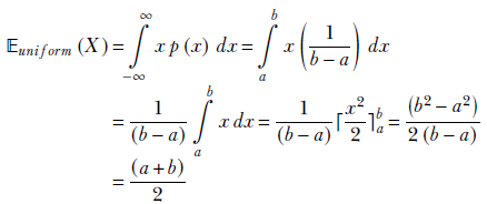
Equation 5.18
NOTE The limits of integration changed because p(x) is zero outside the interval [a, b].
Overall, equation 5.18 agrees with our intuition. The expected value is right in the middle of the uniform interval, as shown in figure 5.5.
Variance of a uniform distribution
If we look at figure 5.5, it is intuitively obvious that the packing density of the samples is related to the width of the rectangle. The smaller the width, the tighter the packing and the smaller the variance, and vice versa. Let’s see if the math supports that intuition:
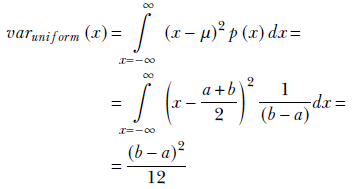
Equation 5.19
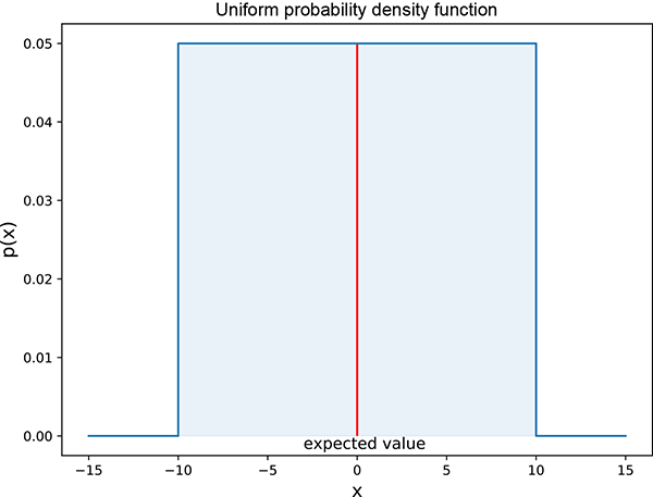
Figure 5.5 Univariate (single-variable) uniform random probability density function. The solid line in the middle indicates the expected value. Interactive visualizations (where ou can change the parameters and observe how the graph changes as a result) can be found at http://mng.bz/E2Jr.
Figure 5.5 shows that the variance in equation 5.19 is proportional to the square of the width of the rectangle: that is, (b − a)2.
Here is the PyTorch code for the mean and variance of a uniform random distribution.
Listing 5.2 Mean and variance of a uniform random distribution
num_samples = 100000                              ①

    ②
samples  = ufm_dist.sample([num_samples])         ③


sample_mean = samples.mean()                      ④
dist_mean = ufm_dist.mean                         ⑤
assert torch.isclose(sample_mean, dist_mean, atol=0.2)

sample_var = ufm_dist.sample([num_samples]).var() ⑥
dist_var = ufm_dist.variance                      ⑦
assert torch.isclose(sample_var, dist_var, atol=0.2)
① Number of sample points
② 100000 × 1
③ Obtains samples from ufm_dist instantiated in listing 5.1
④ Sample mean
⑤ Mean via PyTorch function
⑥ Sample variance
⑦ Variance via PyTorch function
Multivariate uniform distribution
Uniform distributions also can be multivariate. In that case, the random variable is a vector, ![]() not a single value, but a sequence of values). Its domain is a multidimensional volume instead of the X-axis, and the graph has more than two dimensions. For example, this is a two-variable uniform random distribution:
not a single value, but a sequence of values). Its domain is a multidimensional volume instead of the X-axis, and the graph has more than two dimensions. For example, this is a two-variable uniform random distribution:
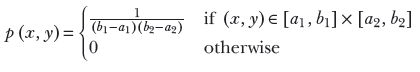
Equation 5.20
Here, (x, ![]() ) ∈ [a1, b1] × [a2, b2] indicates a rectangular domain on the two-dimensional XY plane where x lies between a1 and b1 and
) ∈ [a1, b1] × [a2, b2] indicates a rectangular domain on the two-dimensional XY plane where x lies between a1 and b1 and ![]() lies between a2 and b2. Equation 5.20 is shown graphically in figure 5.6. In the general multidimensional case,:
lies between a2 and b2. Equation 5.20 is shown graphically in figure 5.6. In the general multidimensional case,:
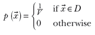
Equation 5.21
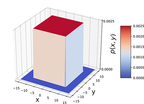
Figure 5.6 Bivariate uniform random probability density The probability p(x, y) is constant, 0.0025, in the domain (x, y) ∈ [−10,10] × [−10,10] and zero everywhere outside the interval. The volume of the box of width 20 × 20 and height 0.0025, 20 * 20 * 0.0025 = 1.
Here, V is the volume of the hyperdimensional box with base D. Equation 5.21 means p(![]() ) is constant for
) is constant for ![]() in the domain D and zero for other values of x. When nonzero, it has a constant value, the inverse of the volume V: this makes the total volume under the density function 1.
in the domain D and zero for other values of x. When nonzero, it has a constant value, the inverse of the volume V: this makes the total volume under the density function 1.
5.9.2 Gaussian (normal) distribution
This is probably the most famous distribution in the world. Let’s consider, one more time, the weights of adult residents of Statsville. If Statsville is anything like a real city, the likeliest weight is around 75 kg: the largest percentage of the population will weigh this much. Weights near this value (say 70 or 80 kg) will also be quite likely, although slightly less likely than 75 kg. Weights further away from 75 kg are still less likely, and so on. The further we go from 75 kg, the lower the percentage of the population with that weight. Outlier values like 40 and 110 kg are unlikely. Informally speaking, a Gaussian probability density function looks like a bell-shaped curve. The central value has the highest probability. The probability falls gradually as we move away from the center. In theory, however, it never disappears completely (the function p(x) never becomes equal to 0), although it becomes almost zero for all practical purposes. This behavior is described in mathematics as asymptotically approaching zero. Figure 5.7 shows a Gaussian probability density function. Formally,
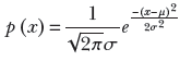
Equation 5.22
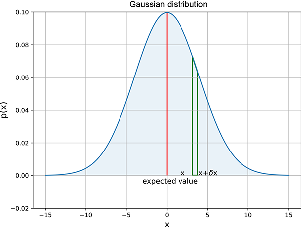
Figure 5.7 Univariate Gaussian random probability density function, μ = 0 and σ = 4. The bell-shaped curve is highest at the center and decreases more and more as we move away from the center, approaching zero asymptotically. The value x = 0 has the highest probability, corresponding to the center of the probability density function. Note that the curve is symmetric. Thus, for instance, the probability of a random sample being in the vicinity of −5 is the same as that of 5 (0.04): that is, p(−5) = p(5) = 0.04. An interactive visualization (where you can change the parameters and observe how the graph changes as a result) can be found at http://mng.bz/NYJX.
Here, μ and σ are parameters; μ corresponds to the center (for example, in figure 5.7, μ = 0). The parameter σ controls the width of the bell. A larger σ implies that p(x) falls more slowly as we move away from the center.
The Gaussian (normal) probability density function is so popular that we have a special symbol for it: 𝒩(x, μ, σ2). It can be proved (but doing so is exceedingly tedious, so we will skip the proof here) that
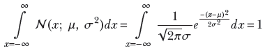
This establishes that 𝒩(x;μ, σ2) is a true probability (satisfying the sum rule in equation 5.7).
Listing 5.3 Log probability of a univariate normal distribution
from torch.distributions import Normal        ①

mu = torch.tensor([0.0], dtype=torch.float)   ②
sigma = torch.tensor([5.0], dtype=torch.float)

uvn_dist = Normal(mu, sigma)                  ③

X = torch.tensor([0.0], dtype=torch.float)    ④

def raw_eval(X, mu, sigma):
    K = 1 / (math.sqrt(2 * math.pi) * sigma)
    E = math.exp( -1 * (X - mu) ** 2 * (1 / (2 * sigma ** 2)))
    return math.log(K * E)

log_prob = uvn_dist.log_prob(X)               ⑤
raw_eval_log_prob = raw_eval(X, mu, sigma)    ⑥
assert log_prob == raw_eval_log_prob          ⑦
① Imports a PyTorch univariate normal distribution
② Sets the distribution params
③ Instantiates a univariate normal distribution object
④ Instantiates a single-point test dataset
⑤ Evaluates the probability using PyTorch
⑥ Evaluates the probability using the formula
⑦ Asserts that the probabilities match
NOTE Fully functional code for this normal distribution, executable via Jupyter Notebook, can be found at http://mng.bz/NYJX.
Multivariate Gaussian
A Gaussian distribution can also be multivariate. Then the random variable x is a vector ![]() , as usual. The parameter μ also becomes a vector
, as usual. The parameter μ also becomes a vector ![]() , and the parameter σ becomes a matrix Σ. As in the univariate case, these parameters are related to the expected value and variance. The Gaussian multivariate probability distribution function is
, and the parameter σ becomes a matrix Σ. As in the univariate case, these parameters are related to the expected value and variance. The Gaussian multivariate probability distribution function is
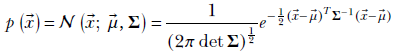
Equation 5.23
Equation 5.23 describes the probability density function for the random vector ![]() to lie within the infinitesimally small volume with dimensions δ
to lie within the infinitesimally small volume with dimensions δ![]() around the point
around the point ![]() . (Imagine a tiny box (cuboid) whose sides are successive elements of δ
. (Imagine a tiny box (cuboid) whose sides are successive elements of δ![]() , with the top-left corner of the box at
, with the top-left corner of the box at ![]() .) The vector
.) The vector ![]() and the matrix Σ are parameters. As in the univariate case,
and the matrix Σ are parameters. As in the univariate case, ![]() corresponds to the most likely value of the random vector. Figure 5.8 shows the Gaussian normal) distribution with two variables in three dimensions. The shape of the base of the bell is controlled by the parameter Σ.
corresponds to the most likely value of the random vector. Figure 5.8 shows the Gaussian normal) distribution with two variables in three dimensions. The shape of the base of the bell is controlled by the parameter Σ.
Listing 5.4 Log probability of a multivariate normal distribution
from torch.distributions import MultivariateNormal ①

mu = torch.tensor([0.0, 0.0], dtype=torch.float)   ②
C = torch.tensor([[5.0, 0.0], [0.0, 5.0]], dtype=torch.float)

mvn_dist = MultivariateNormal(mu, C)               ③

X = torch.tensor([0.0, 0.0], dtype=torch.float)    ④

def raw_eval(X, mu, C):
    K = (1 / (2 * math.pi * math.sqrt(C.det())))
    X_minus_mu = (X - mu).reshape(-1, 1)
    E1 = torch.matmul(X_minus_mu.T, C.inverse())
    E = math.exp(-1 / 2. * torch.matmul(E1, X_minus_mu))
    return math.log(K * E)

log_prob = mvn_dist.log_prob(X)                    ⑤
raw_eval_log_prob = raw_eval(X, mu, C)             ⑥
assert log_prob == raw_eval_log_prob               ⑦
① Imports a PyTorch multivariate normal distribution
② Sets the distribution params
③ Instantiates a multivariate normal distribution object
④ Instantiates a single point test dataset
⑤ Evaluates the probability using PyTorch
⑥ Evaluates the probability using the formula
⑦ Asserts that the probabilities match
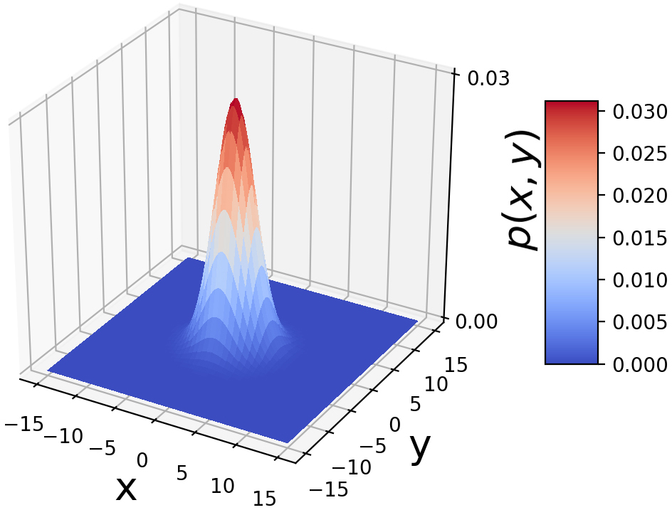
Figure 5.8 Bivariate Gaussian random probability density function. It is a bell-shaped surface: highest at the center and decreasing as we move away from the center, approaching zero asymptotically. x = 0, ![]() = 0 has the highest probability, corresponding to the center of the probability density function. The bell has a circular base, and the Σ matrix is a scalar multiple of the identity matrix 𝕀. An interactive visualization (where you can change the parameters and observe how the graph changes as a result) can be found at http://mng.bz/NYJX.
= 0 has the highest probability, corresponding to the center of the probability density function. The bell has a circular base, and the Σ matrix is a scalar multiple of the identity matrix 𝕀. An interactive visualization (where you can change the parameters and observe how the graph changes as a result) can be found at http://mng.bz/NYJX.
Expected value of a Gaussian distribution
Substituting the probability density function from equation 5.22 into the expression for the expected value of a continuous variable, equation 5.10, we get
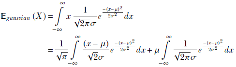
Substituting ![]()
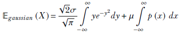
Substituting u = y2 and using equation 5.6
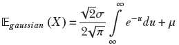
Note that the limits of the integral in the first term are identical. This is because u = y2 →∞ whether y → ∞ or y → −∞. But an integral with the same lower and upper limits is zero. Thus the first term is zero. Hence,
𝔼gaussian(X) = μ
Equation 5.24
Intuitively, this makes perfect sense. The probability density ![]() peaks (maximizes) at x = μ. At this x, the exponent becomes zero, which makes the term
peaks (maximizes) at x = μ. At this x, the exponent becomes zero, which makes the term ![]() attain its maximum possible value of 1. This is right in the middle of the bell, as shown in figure 5.10. And, of course, the expected value coincides with the middle value if the density is symmetric and peaks in the middle. Analogously, in the multivariate case, the Gaussian multidimensional random variable X that takes vector values
attain its maximum possible value of 1. This is right in the middle of the bell, as shown in figure 5.10. And, of course, the expected value coincides with the middle value if the density is symmetric and peaks in the middle. Analogously, in the multivariate case, the Gaussian multidimensional random variable X that takes vector values ![]() in the d-dimensional domain ℝd (that is,
in the d-dimensional domain ℝd (that is, ![]() ∈ ℝd) has an expected value
∈ ℝd) has an expected value
𝔼gaussian(X) = ![]()
Equation 5.25
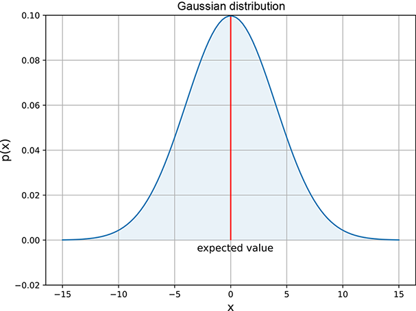
Figure 5.9 Univariate (single-variable) normal (Gaussian) random probability density function, μ = 0 and σ = 4. The solid line in the middle indicates the expected value.
Variance of a Gaussian distribution
The variance of the Gaussian distribution is obtained by substituting equation 5.22 in the integral form of equation 5.13. The mathematical derivation is shown in the book’s appendix; here we only state the result.
The variance of a Gaussian distribution with probability density function ![]() is σ2, and the standard deviation is the square root of that (σ). This makes intuitive sense. σ appears in the denominator of a negative exponent in the expression for the probability density function
is σ2, and the standard deviation is the square root of that (σ). This makes intuitive sense. σ appears in the denominator of a negative exponent in the expression for the probability density function ![]() . As such, p(x) is an increasing function of σ: that is, for a given x and μ, a larger σ implies a larger p(x). In other words, a larger σ implies that the probability decays more slowly as we move away from the center: a fatter bell curve, a bigger spread, and hence a larger variance. Figure 5.10 depicts this.
. As such, p(x) is an increasing function of σ: that is, for a given x and μ, a larger σ implies a larger p(x). In other words, a larger σ implies that the probability decays more slowly as we move away from the center: a fatter bell curve, a bigger spread, and hence a larger variance. Figure 5.10 depicts this.
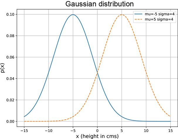
(a) Different μs but the same σs.
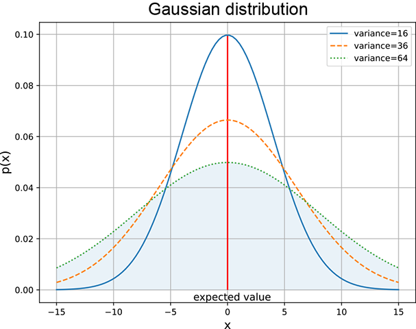
(b) The same μs but different σs.
Figure 5.10 Gaussian densities with varying μs and σs. Changing μ shifts the center of the curve. A larger σ (variance) implies a fatter bell ⇒ more spread. Note that fatter curves are smaller in height as the total area under the curve must be 1.
Listing 5.5 Mean and variance of a univariate Gaussian
num_samples = 100000                              ①

    ②
samples  = uvn_dist.sample([num_samples])         ③


sample_mean = samples.mean()                      ④
dist_mean = uvn_dist.mean                         ⑤
assert torch.isclose(sample_mean, dist_mean, atol=0.1)

sample_var = uvn_dist.sample([num_samples]).var() ⑥
dist_var = uvn_dist.variance                      ⑦
assert torch.isclose(sample_var, dist_var, atol=0.1)
① Number of sample points
② 100000 × 1
③ Obtains samples from uvn_dist
instantiated in listing 5.3
④ Sample mean
⑤ Mean via PyTorch function
⑥ Sample variance
⑦ Variance via PyTorch function
Covariance of a multivariate Gaussian distribution and geometry of the bell surface
Comparing equation 5.22 for a univariate Gaussian probability density with equation 5.23 for a multivariate Gaussian probability density, we intuitively feel that the matrix Σ is the multivariate peer of the univariate variance σ2. Indeed it is. Formally, for a multivariate Gaussian random variable with a probability distribution given in equation 5.23, the covariance matrix is given by the equation
ℂgaussian(X) = Σ
Equation 5.26
As shown in table 5.11, Σ regulates the shape of the base of the bell-shaped probability density function.
It is easy to see that the exponent in equation 5.23 is a quadratic form (introduced in section 4.2). As such, it defines a hyper-ellipse, as shown in figure 5.11 and section 2.17. All the properties of quadratic forms and hyper-ellipses apply here.
Listing 5.6 Mean and variance of a multivariate normal distribution
num_samples = 100000                              ①

    ②
samples  = mvn_dist.sample([num_samples])         ③


sample_mean = samples.mean()                      ④
dist_mean = mvn_dist.mean                         ⑤
assert torch.allclose(sample_mean, dist_mean, atol=1e-1)

sample_var = mvn_dist.sample([num_samples]).var() ⑥
dist_var = mvn_dist.variance                      ⑦
assert torch.allclose(sample_var, dist_var, atol=1e-1)
① Number of sample points
② 100000 × 1
③ Obtains samples from uvn_dist
instantiated in listing 5.4
④ Sample mean
⑤ Mean via PyTorch function
⑥ Sample variance
⑦ Variance via PyTorch function
Let’s look at the geometric properties of the Gaussian covariance matrix Σ. Consider a 2D version of equation 5.23. We rewrite ![]() and
and ![]() —2D vectors both. Also
—2D vectors both. Also ![]() —a 2 × 2 matrix. The probability density function from equation 5.23 becomes
—a 2 × 2 matrix. The probability density function from equation 5.23 becomes
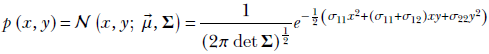
Equation 5.27
(Use what you learned in chapter 3 to satisfy yourself that equation 5.27 is a 2D analog of equation 5.23.)
If we plot the surface p(x, y) against (x, y), it looks like a bell in 3D space. The shape of the bell’s base, on the (x, y) plane, is governed by the 2 × 2 matrix Σ. In particular,
-
If Σ is a diagonal matrix with equal diagonal elements, the bell is symmetric in all directions, and its base is circular.
-
If Σ is a diagonal matrix with unequal diagonal elements, the base of the bell is elliptical. The axes of the ellipse are aligned with the coordinate axes.
-
For a general Σ matrix, the base of the bell is elliptical. The axes of the ellipse are not necessarily aligned with the coordinate axes.
-
The eigenvectors of Σ yield the axes of the elliptical base of the bell surface.
Now, if we sample the distribution from equation 5.27, we get a set of points (x, y) on the base plane of the surface shown in figure 5.8. The taller the z coordinate (depicting p(x, y)) of the surface at a point (x, y), the greater its probability of being selected in the sampling. If we draw a large number of samples, the corresponding point cloud will look more or less like the base of the bell surface.
Figure 5.11 shows various point clouds formed by sampling Gaussian distributions with different covariance matrices Σ. Compare it to figure 5.10.
Geometry of sampled point clouds: Covariance and direction of maximum or minimum spread
We have seen that if a multivariate distribution has a covariance matrix ℂ, its variance (spread) in any specific direction l̂ is l̂T ℂl̂. What is the direction of maximum spread?
Asking this is the same as asking “What direction l̂ maximizes the quadratic form l̂T ℂl̂?” In section 4.2, we saw that a quadratic form like this is maximized or minimized when the direction l̂ is aligned with the eigenvector corresponding to the maximum or minimum eigenvalue of the matrix ℂ. Thus, the maximum spread of a distribution occurs along the eigenvector of the covariance matrix corresponding to its maximum eigenvalue. This led to the PCA technique in section 4.4.
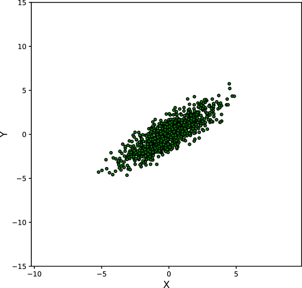
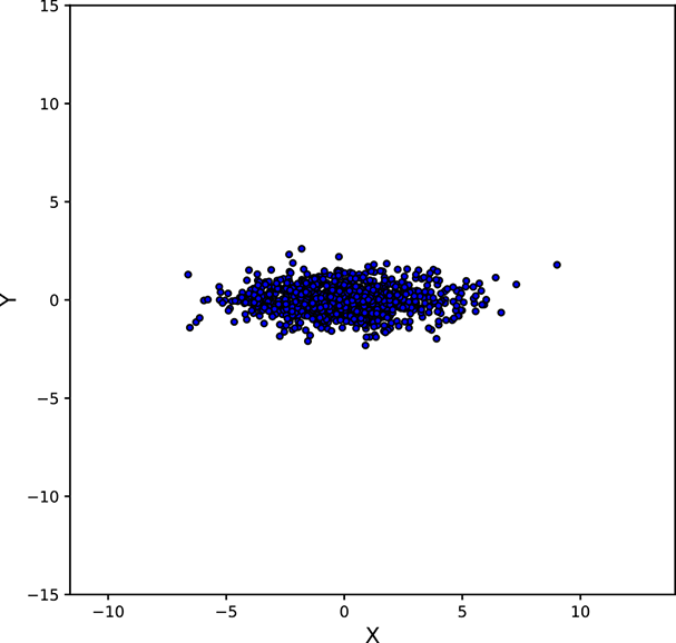
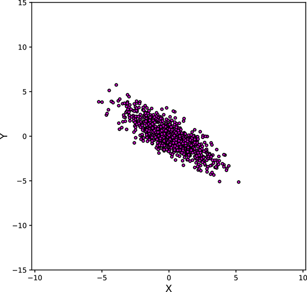
Next, we discuss the covariance of the Gaussian distribution and geometry of the point cloud formed by sampling a multivariate Gaussian a large number of times. You may want to take a look at figure 5.11, which shows various point clouds formed by sampling Gaussian distributions with different covariance matrices Σ.
(a) ![]()
(b) ![]()
(c) ![]()
(d) ![]()
Figure 5.11 Point clouds formed by sampling multivariate Gaussians with the same ![]() = [0,0]T but different Σs. These point clouds correspond to the bases of the bell curves for multivariate Gaussian probability densities. All the point clouds except (a) may be replaced by a univariate Gaussian after rotation to align the coordinate axes with the eigenvectors of Σ (dimensionality reduction). See sections 4.4, 4.5, and 4.6 for details. Interactive contour plots for the base of the bell curve can be found at http://mng.bz/NYJX.
= [0,0]T but different Σs. These point clouds correspond to the bases of the bell curves for multivariate Gaussian probability densities. All the point clouds except (a) may be replaced by a univariate Gaussian after rotation to align the coordinate axes with the eigenvectors of Σ (dimensionality reduction). See sections 4.4, 4.5, and 4.6 for details. Interactive contour plots for the base of the bell curve can be found at http://mng.bz/NYJX.
Multivariate Gaussian point clouds and hyper-ellipses
The numerator of the exponential term in equation 5.23, (![]() −
−![]() )TΣ−1(
)TΣ−1(![]() −
−![]() ), is a quadratic form as we discussed in section 4.2. It should also remind you of the hyper-ellipse we looked at in section 2.17, equation 2.33, and equation 4.1.
), is a quadratic form as we discussed in section 4.2. It should also remind you of the hyper-ellipse we looked at in section 2.17, equation 2.33, and equation 4.1.
Now consider the plot of p(![]() ) against
) against ![]() . This is a hypersurface in n + 1-dimensional space, where the random variable
. This is a hypersurface in n + 1-dimensional space, where the random variable ![]() is n-dimensional. For instance, if the random Gaussian variable
is n-dimensional. For instance, if the random Gaussian variable ![]() is 2D, the (
is 2D, the (![]() , p(
, p(![]() )) plot in 3D is as shown in figure 5.8. It is a bell-shaped surface. The hyper-ellipse corresponding to the quadratic form in the numerator of the probability density function in equation 5.23 governs the shape and size of the base of this bell.
)) plot in 3D is as shown in figure 5.8. It is a bell-shaped surface. The hyper-ellipse corresponding to the quadratic form in the numerator of the probability density function in equation 5.23 governs the shape and size of the base of this bell.
If the matrix Σ is diagonal (with equal diagonal elements), the base is circular—this is the special case shown in figure 5.8. Otherwise, the base of the bell is elliptic. The eigenvectors of the covariance matrix Σ correspond to the directions of the axes of the elliptical base. The eigenvalues correspond to the lengths of the axes.
5.9.3 Binomial distribution
Suppose we have a database containing photos of people. Also, suppose we know that 20% of the photos contain a celebrity and the remaining 80% do not. If we randomly select three photos from this database, what is the probability that two of them contain a celebrity? This is the kind of problem the binomial distribution deals with.
In a computer vision-centric machine learning setting, we would probably inspect the selected photos and try to predict whether they contained a celebrity. But for now, let’s restrict ourselves to the simpler task of blindly predicting the chances from aggregate statistics.
If we select a single photo, the probability of it containing a celebrity is π = 0.2.
NOTE This has nothing to do with the natural number π denoting the ratio of the circumference to the diameter of a circle. We are just reusing the symbol π following popular convention.
The probability of the photo not containing a celebrity is 1 − π = 0.8. From that, we can compute the probability of, say, the first two sampled photos containing a celebrity but the last one containing a non-celebrity: that is, the event {S, S, F} (where S denotes success in finding a celebrity and F denotes failure in finding a celebrity). Using equation 5.4, the probability of the event {S, S, F} is π × π × (1−π) = 0.2 × 0.2 × 0.8. However, many other combinations are also possible.
All the possible combinations that can occur in three trials are shown in table 5.8. In the table, event ids 3, 5, and 6 correspond to two successes and one failure. They occur with probabilities 0.8 × 0.2 × 0.2, 0.2 × 0.8 × 0.2, and 0.2 × 0.2 × 0.8, respectively. If any one of them occurs, we have two celebrity photos in three trials. Thus, using equation 5.3, the overall probability of selecting two celebrity photos in three trials is the sum of these event probabilities: 0.8 × 0.2 × 0.2 + 0.2 × 0.8 × 0.2 + 0.2 × 0.2 × 0.8 = 0.096.
Table 5.8 All possible combinations of three trials
|
Event Id |
Event |
Probability |
|---|---|---|
|
0 |
{F, F, F} |
(1−π) × (1−π) × (1−π) = 0.8 × 0.8 × 0.8 |
|
1 |
{F, F, S} |
(1−π) × (1−π) × π = 0.8 × 0.8 × 0.2 |
|
2 |
{F, S, F} |
(1−π) × π × (1−π) = 0.8 × 0.2 × 0.8 |
|
3 |
{F, S, S} |
(1−π) × π × π = 0.8 × 0.2 × 0.2 |
|
4 |
{S, F, F} |
π × (1−π) × (1−π) = 0.2 × 0.8 × 0.8 |
|
5 |
{S, F, S} |
π × (1−π) × π = 0.2 × 0.8 × 0.2 |
|
6 |
{S, S, F} |
π × π × (1−π) = 0.2 × 0.2 × 0.8 |
|
7 |
{S, S, S} |
π × π × π = 0.2 × 0.2 × 0.2 |
In the general case, with more than three trials, it would be impossibly tedious to enumerate all the possible combinations of success and failure that can occur in a set of n trials. Fortunately, we can derive a formula. But before doing that, let’s state the task of a binomial distribution in more general terms:
Given a process that has a binary outcome (success or failure) in any given trial, and given that the probability of success in a trial is a known constant (say, π), a binomial distribution deals with the probability of observing k successes in n trials of the process.
Imagine events with n successive items, where each individual item can be either S or F. Table 5.8 shows such events with n = 3. Each item has two possible values (S or F), and there are n items. Hence, altogether there can be 2 × 2 × ⋯2 = 2n possible events.
We are only interested in events with k occurrences of S (and therefore (n − k) occurrences of F). How many of the n events are like that? Well, asking this is the same as asking how many ways we can choose k slots from a total of n possible slots. Another way to pose the same question is, “How many different orderings of n items exist, where each item is either S or F and the total count of S is k?” The answer, from combination theory, is
Each of these events has a probability of πk × (1−π)n − k. Hence, the overall probability of k successes in n trials is ![]() .
.
Formally, if X is a random variable denoting the number of successes in n trials, with the probability of success in any single trial being some constant value π,
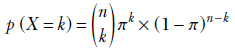
Equation 5.28
What values can k take? Of course, we cannot have more than n successes in n trials; therefore, the maximum possible value of k is n. All integer values between 0 and n are possible:
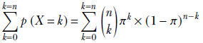
The right-hand side is an expression for the generic term in the famous binomial expansion of (a + b)n with a = π and b = 1 − π. Hence, we get
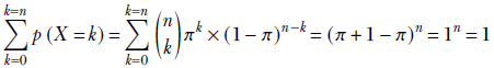
Equation 5.29
This agrees with intuition, since given n, k can only take values 0, 1, ⋯, n; the sum of the probabilities on the left-hand side of equation 5.29 corresponds to a certain event with probability 1.
Also, plugging n = 3, k = 2, and π = 0.2 into equation 5.28 yields 3!/2!1! (0.2)2, (0.8)3-2 = 0.096: exactly what we get from explicit enumeration.
Listing 5.7 Log probability of a binomial distribution
from torch.distributions import Binomial                     ①

num_trials = 3                                               ②
p = torch.tensor([0.2], dtype=torch.float)

binom_dist = Binomial(num_trials, probs=p)                   ③

X = torch.tensor([1], dtype=torch.float)                     ④

def nCk(n, k):
    f = math.factorial
    return f(n) * 1. / (f(k) * f(n-k))

def raw_eval(X, n, p):
    result = nCk(n, X) * (p ** X) * (1 - p) ** (n - X)
    return torch.log(result)

log_prob = binom_dist.log_prob(X)                            ⑤
raw_eval_log_prob = raw_eval(X, num_trials, p)               ⑥
assert torch.isclose(log_prob, raw_eval_log_prob, atol=1e-4) ⑦
① Imports a PyTorch binomial distribution
② Sets the distribution params
③ Instantiates a binomial distribution object
④ Instantiates a single point test dataset
⑤ Evaluates the probability using PyTorch
⑥ Evaluates the probability using formula
⑦ Asserts that the probabilities match
NOTE Fully functional code for the binomial distribution, executable via Jupyter Notebook, can be found at http://mng.bz/DRJ0.
Expected value of a binomial distribution
We have seen that the binomial distribution deals with a random variable X that depicts the number of successes in n trials, where the probability of success in a given trial is a constant π (again, this has nothing to do with the π denoting the ratio of the circumference to the diameter of a circle). This X can take any integer value 0 to n. Hence,

We can drop the first term, which has the multiplier k = 0. Thus we get
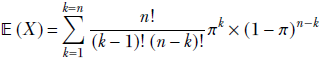
We can factor n! = n(n − 1)! and πk = π πk − 1. Also, n − k = (n − 1) − (k − 1). This gives us
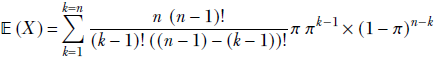
Substituting j for k − 1 and m for n − 1, we get
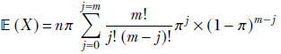
Equation 5.30
The quantity within the summation is similar to that in equation 5.29 (should sum to 1). This leaves us with
𝔼binomial (X) = nπ
Equation 5.31
Equation 5.31 says that if π is the probability of success in a single trial, then the expected number of successes in n trials is nπ. For instance, if the probability of success in a single trial is 0.2, then the expected number of successes in 100 trials is 20—which is almost intuitively obvious.
Variance of a binomial distribution
The variance of a binomial random variable depicting the number of successes in n trials where the probability of success in a given trial is a constant π is
varbinomial = nπ (1 − π)
Equation 5.32
The proof follows the same lines as that of the expected value.
Listing 5.8 Mean and variance of a binomial distribution
num_samples = 100000                                ①

   ②
samples  = binom_dist.sample([num_samples])         ③


sample_mean = samples.mean()                        ④
dist_mean = binom_dist.mean                         ⑤
assert torch.isclose(sample_mean, dist_mean, atol=0.2)

sample_var = binom_dist.sample([num_samples]).var() ⑥
dist_var = binom_dist.variance                      ⑦
assert torch.isclose(sample_var, dist_var, atol=0.2)
① Number of sample points
② 100000 × 1
③ Obtains samples from ufm_dist instantiated in listing 5.7
④ Sample mean
⑤ Mean via PyTorch function
⑥ Sample variance
⑦ Variance via PyTorch function
5.9.4 Multinomial distribution
Consider again the example problem we discussed in section 5.9.3. We have a database of photos of people. But instead of two classes, celebrity and non-celebrity, we have four classes:
-
Photos of Albert Einstein (class 1): 10% of the photos
-
Photos of Marie Curie (class 2): 42% of the photos
-
Photos of Carl Friedrich Gauss (class 3): 4% of the photos
-
Other photos (class 4): 44% of the photos
If we randomly select a photo from the database (that is, perform a random trial),
-
The probability of selecting class 1 (picking an Einstein photo) is π1 = 0.1.
-
The probability of selecting class 2 (picking a Marie Curie photo) is π2 = 0.42.
-
The probability of selecting class 3 (picking a Gauss photo) is π3 = 0.04.
-
The probability of selecting class 4 (picking a photo of none of the above) is π4 = 0.44.
Notice that π1 + π2 + π3 + π4 = 1. This is because the classes are mutually exclusive and exhaustive, so exactly one of these classes must occur in every trial.
Given all this, let’s ask the question: “What is the probability that in a set of 10 random trials, class 1 occurs 1 time, class 2 occurs 2 times, class 3 occurs 1 time, and class 4 occurs the remaining 6 times?” This is the kind of problem multinomial distributions deal with.
Formally,
-
Let C1, C2, ⋯, Cm be a set of m classes such that in any random trial, exactly one of these classes will be selected with the respective probabilities π1, π2, ⋯, πm.
-
Let X1, X2, ⋯, Xm be a set of random variables. Xi corresponds to the number of occurrences of class Ci in a set of n trials.
-
Then the multinomial probability function depicting the probability that class C1 is selected k1 times, class C2 is selected k2 times, and class C3 is selected km times is
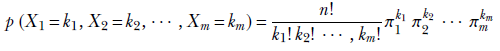
Equation 5.33
where
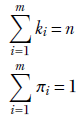
We can verify that for m = 2, this becomes the binomial distribution (equation 5.28). A noteworthy point is that if we look at any one of the m variables X1, X2, ⋯, Xm individually, its distribution is binomial.
Let’s work out the final probability for the example we started with: the probability that in a set of 10 random trials, class 1 occurs 1 time, class 2 occurs 2 times, class 3 occurs 1 time, and class 4 occurs the remaining 6 times. This is

Listing 5.9 Log probability of a multinomial distribution
from torch.distributions import Multinomial                  ①

num_trials = 10                                              ②
P = torch.tensor([0.1, 0.42, 0.04, 0.44], dtype=torch.float)

multinom_dist = Multinomial(num_trials, probs=P)             ③

X = torch.tensor([1, 2, 1, 6], dtype=torch.float)            ④

def raw_eval(X, n, P):
    f = math.factorial
    result = f(n)
    for p, x in zip(P, X):
        result *= (p ** x) / f(x)
    return math.log(result)

log_prob = multinom_dist.log_prob(X)                         ⑤
raw_eval_log_prob = raw_eval(X, num_trials, P)               ⑥
assert torch.isclose(log_prob, raw_eval_log_prob, atol=1e-4) ⑦
① Imports a PyTorch multinomial distribution
② Sets the distribution params
③ Instantiates a multinomial dist object
④ Instantiates a single-point test dataset
⑤ Evaluates the probability using PyTorch
⑥ Evaluates the probability using formula
⑦ Asserts that the probabilities match
NOTE Fully functional code for the multinomial distribution, executable via Jupyter Notebook, can be found at http://mng.bz/l1gz.
Expected value of a multinomial distribution
Each of the random variables X1, X2, ⋯, Xm individually subscribes to a binomial distribution. Accordingly, following the binomial distribution expected value formula from equation 5.31,
𝔼multinomial(Xi) = nπi
Equation 5.34
Variance of a multinomial distribution
The variation of the random variables X1, X2, ⋯, Xm, following the binomial distribution variance formula from equation 5.32, is
varmultinomial(Xi) = nπi(1−πi)
Equation 5.35
If each of the X1, X2, ⋯, Xm is a scalar, then we can think of a random vector ![]() . The expected value of such a random variable is
. The expected value of such a random variable is
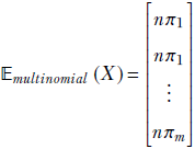
and the covariance is
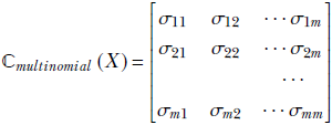
Equation 5.36
where the diagonal terms are like the binomial variance σii = nπi(1−πi) ∀i ∈ [1, m] and the off-diagonal terms are σij = −nπiπj ∀(i, j) ∈ [1, m] × [1, m]. The cross-covariance terms in the diagonal are negative because an increase in one element implies a decrease in the others.
Listing 5.10 Mean and variance of a multinomial distribution
num_samples = 100000                                         ①

   ②
samples = multinom_dist.sample([num_samples])                ③

sample_mean = samples.mean(axis=0)                           ④
dist_mean = multinom_dist.mean                               ⑤
assert torch.allclose(sample_mean, dist_mean, atol=0.2)

sample_var = multinom_dist.sample([num_samples]).var(axis=0) ⑥
dist_var = multinom_dist.variance                            ⑦
assert torch.allclose(sample_var, dist_var, atol=0.2)
① Number of sample points
② 100000 × 1
③ Obtains samples from ufm_dist instantiated in listing 5.9
④ Sample mean
⑤ Mean via PyTorch function
⑥ Sample variance
⑦ Variance via PyTorch function
5.9.5 Bernoulli distribution
A Bernoulli distribution is a special case of a binomial distribution where n = 1: that is, a single success-or-failure trial is performed. The probability of success is π, and the probability of failure is 1 − π.
In other words, let X be a discrete random variable that takes the value 1 (success) with probability π and the value 0 (failure) with probability 1 − π. The distribution of X is the Bernoulli distribution:
p(X = 1) = π
p(X = 0) = 1 - π
Listing 5.11 Log probability of a Bernoulli distribution
from torch.distributions import Bernoulli                    ①

p = torch.tensor([0.3], dtype=torch.float)                   ②

bern_dist = Bernoulli(p)                                     ③
X = torch.tensor([1], dtype=torch.float)                     ④
def raw_eval(X, p):
    prob = p if X == 1 else 1-p
    return math.log(prob)

log_prob = bern_dist.log_prob(X)                             ⑤
raw_eval_log_prob = raw_eval(X, p)                           ⑥
assert torch.isclose(log_prob, raw_eval_log_prob, atol=1e-4) ⑦
① Imports a PyTorch Bernoulli distribution
② Sets the distribution params
③ Instantiates a Bernoulli distribution object
④ Instantiates a single-point test dataset
⑤ Evaluates the probability using PyTorch
⑥ Evaluates the probability using the formula
⑦ Asserts that the probabilities match
NOTE Fully functional code for the Bernoulli distribution, executable via Jupyter Notebook, can be found at http://mng.bz/BRwq.
Expected value of a Bernoulli distribution
If there are only two classes, success and failure, we cannot speak directly of an expected value. If we run, say, 100 trials and get 30 successes and 70 failures, the average is 0.3 success, which is not a valid outcome. We cannot have fractional success or failure in this binary system.
We can, however, talk about the expected value of a Bernoulli distribution if we introduce an artificial construct. We assign numerical values to these binary entities: success = 1 and failure = 0. Then the expected value of X is
![]()
Equation 5.37
Variance of a Bernoulli distribution
Similarly, if we assign numerical values to these binary entities—success = 1 and failure = 0—the variance of the Bernoulli distribution is

Equation 5.38
Listing 5.12 Mean and variance of a Bernoulli distribution
num_samples = 100000                               ①

   ②
samples = bern_dist.sample([num_samples])          ③

sample_mean = samples.mean()                       ④
dist_mean = bern_dist.mean                         ⑤
assert torch.isclose(sample_mean, dist_mean, atol=0.2)

sample_var = bern_dist.sample([num_samples]).var() ⑥
dist_var = bern_dist.variance                      ⑦
assert torch.isclose(sample_var, dist_var, atol=0.2)
① Number of sample points
② 100000 × 1
③ Obtains samples from ufm_dist instantiated in listing 5.11
④ Sample mean
⑤ Mean via PyTorch function
⑥ Sample variance
⑦ Variance via PyTorch function
5.9.6 Categorical distribution and one-hot vectors
Consider again the example problem introduced in section 5.9.4. We have a database with four classes of photos:
-
Photos of Albert Einstein (class 1): 10%
-
Photos of Marie Curie (class 2): 42%
-
Photos of Carl Friedrich Gauss (class 3): 4%
-
Other photos (class 4): 44%
If we randomly select a photo from the database,
-
The probability of selecting class 1 is π1 = 0.1.
-
The probability of selecting class 2 is π2 = 0.42.
-
The probability of selecting class 3 is π3 = 0.04.
-
The probability of selecting class 4 is π4 = 0.44.
As before, π1 + π2 + π3 + π4 = 1 because the classes are mutually exclusive and exhaustive so exactly one class must occur in each trial.
In multinomial distribution, we performed n trials and asked how many times each specific class would occur. What if we perform only one trial? Then we get categorical distribution.
Categorical distribution is a special case of multinomial distribution (with the number of trials n = 1). It is also an extension of the Bernoulli distribution where instead of just two classes, success and failure, we can have an arbitrary number of classes.
Formally,
-
Let C1, C2, ⋯, Cm be a set of m classes such that in any random trial, exactly one of these classes will be selected, with the respective probabilities π1, π2, ⋯, πm. We sometimes refer to the probabilities of all the classes together as a vector

-
Let X1, X2, ⋯, Xm be a set of random variables. Xi corresponds to the number of occurrences of class Ci in a set of n trials.
-
Then the categorical probability function depicts the probability of each of the classes C1, C2, and so on, in a single trial.
One-hot vector
We can use a one-hot vector to compactly express the outcome of a single trial of categorical distribution. This is a vector with m elements. Exactly a single element is 1; all other elements are 0. The 1 indicates which of the m possible classes occurred in that specific trial. For instance, in the example with the database of photos, if a Marie Curie photo comes up in a given trial, the corresponding one-hot vector is  .
.
Probability of a categorical distribution
We can think of a one-hot vector X as a random variable with a categorical distribution. Note that each individual class follows a Bernoulli distribution. The probability of class Ci occurring in any given trial is
p(Ci) = πi
We can express the probability distribution of all the classes together compactly
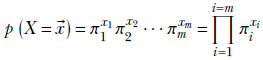
Equation 5.39
where ![]() is a one-hot vector. Note that all but one of the powers in equation 5.39 is 0; hence the corresponding factor evaluates to 1. The remaining power is 1. Hence the overall probability always evaluates to πi, where i is the index of the class that occurred in the trial.
is a one-hot vector. Note that all but one of the powers in equation 5.39 is 0; hence the corresponding factor evaluates to 1. The remaining power is 1. Hence the overall probability always evaluates to πi, where i is the index of the class that occurred in the trial.
Expected value of a categorical distribution
Since we are talking about classes, expected value and variance do not make sense in this context. We encountered a similar situation with the Bernoulli distribution. We assigned numerical values to each class and somewhat artificially defined the expected value and variance. A similar idea can also be applied here: we can talk about the expected value and variance of the one-hot vector (which consists of numerical values 0 and 1). But it remains an artificial construct.
Given a random variable X whose instances are one-hot vectors ![]() following a categorical distribution with m classes with respective probabilities π1, π2, ⋯, πm,
following a categorical distribution with m classes with respective probabilities π1, π2, ⋯, πm,
Equation 5.40
We skip the variance of a categorical distribution.
Summary
In this chapter, we first looked at probability and statistics from a machine learning point of view. We also introduced the PyTorch distributions package and illustrated each concept with PyTorch distributions code samples immediately following the math.
-
The probability of a specific event type is defined as the fraction of the total population of all possible events occupied by events of that specific type.
-
A random variable is a variable that can assume any value from a predefined range of possible values. Random variables can be discrete or continuous. A probability is associated with a discrete random variable taking a specific value. A probability is also associated with a continuous random variable taking a value in an infinitesimally small range around a specific value, called its probability density at that value.
-
The sum rule of probabilities states that the sum of the probabilities of a set of mutually exclusive events is the probability of one or another of them occurring. If the set of events is exhaustive that is, among them, they cover the entire space of possible events), then their sum is 1 because one or another of them must occur. For continuous random variables, integrating the probability density function over the domain of possible values yields 1.
-
The joint probability of a set of events is the probability of all those events occurring together. If the events are independent, the joint probability is the product of their individual probabilities.
-
Drawing a sample from the probability distribution of a random variable returns an arbitrary value from the set of possible values. If we draw many samples, the higher-probability values show up more often than the lower-probability values. The sampled points occupy a region (called the sample point cloud) in the domain of possible values. In a sample point cloud, the region where the probabilities are higher is more densely populated than lower-probability regions.
-
The expected value of a random variable is the average of the values of points in a very large (approaching infinity) sample cloud. It is equal to the weighted sum of all possible values of the random variable, where the weight for each value is its probability of occurrence. For continuous random variables, this boils down to integration—over the domain of possible values—of the product of the random variable’s value and the probability density. The physical significance of the expected value is that it is a single-point representation of the entire distribution.
-
The variance of a random variable is the square root of the average squared distances of the sample point values from the mean in a very large (approaching infinity) sample cloud. It is equal to the weighted sum of the squared distances of all possible values of the random variable from the mean. The weight for each value is its probability of occurrence. For continuous random variables, this boils down to integration—over the domain of possible values—of the product of the squared distance of the random variable’s value from the mean and the probability density. Physically, the variance is a measure of the spread of the points in the distribution around its mean. In the multivariate case, this spread depends on the direction. Since there are infinite possible directions in a space with two or more dimensions, we cannot speak of a single variance value. Instead, we compute a covariance matrix with which to compute the spread along any specified direction. The eigenvector corresponding to the largest eigenvalue of this covariance matrix yields the direction of maximum spread. That eigenvalue yields the maximum spread. The eigenvector corresponding to the next-largest eigenvalue yields the orthogonal direction with the next-highest spread, and so forth.
-
Principal component analysis (PCA) is a technique in multivariate statistics to identify the directions of the maximum spread of data. It uses the eigenvectors and eigenvalues of the covariance matrix.
-
The Gaussian distribution is the most important probability distribution. The Gaussian random variable has one value with the highest probability of occurrence. The probability decreases smoothly with increasing distance from that highest probability value. The probability density function is continuous and looks like a bell-shaped surface. The center of the bell is the highest probability value, which also happens to be the expected value of the Gaussian random variable. The covariance matrix determines the shape of the base of the bell surface. It is circular when the covariance matrix is diagonal, with equal values on the diagonal; it is elliptical in general, with the axes of the ellipse along the eigenvectors of the covariance matrix.
The sample point cloud of a Gaussian distribution is elliptical. It corresponds to the base of the bell-shaped probability density function. The longest spread corresponds to the ellipse’s major axis, which corresponds to the eigenvector corresponding to the largest eigenvalue of the covariance matrix. In the GitHub repository, we have provided an interactive visualizer for observing the shapes of Gaussian distributions in one and two dimensions as you change the parameter values. Take a look at the interactive visualization section at http://mng.bz/NYJX.